Lost in Space I
$\def\sb{_}$ I’d intended to write a long post talking about a bunch of cool stuff I’ve been reading the past month, but Alek told me he thought it might be nicer to have lots of small posts. So here’s the first installment in a series about derandomizing space-bounded algorithms. What started me down this rabbithole was when Ted said offhand something like “for all the work complexity theorists have done, the fanciest explicit PRG we know can only fool algorithms with at most $\log_2(3)$ bits of memory – if you could get this up to $2$ bits, it would be massive result instant FOCS paper”. I thought this was a really funny claim, but then when I went looking to figure out what he meant I realized that it’s actually kinda deep. If you come along for the ride, I’ll tell you the story.
Today, I’ll just talk about how to trick algorithms with only 1 bit of memory.
Small-bias distributions
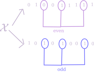
Given some distribution $\mathcal{X}$ on $\lbrace 0,1\rbrace^n$, what’s an easy way to check that output looks close to uniformly random? Well, for every index $i$ you could ask “what’s the probability that the $i$th bit is 1?”, and make sure that’s close to $1/2$. But of course, that’s not enough – what if the string is $000\dots$ half the time and $111\dots$ the other half? To rule this out, you might want to ask “what’s the probability that the $i$th bit is the same as the $j$th bit?”, and make sure that’s close to $1/2$ too. Generalizing this idea, we can define a parity test as follows:
Fix a non-empty subset $S \subseteq [n]$. If I take a sample from $\mathcal{X}$ and look at the parity of the sum of the bits in the $S$th indices, what’s the probability it’ll be odd?

If that probability is at most $\epsilon$ away from $1/2$, we say the test has bias at most $\epsilon$. If, for every $S \subseteq n$, the corresponding parity test has bias at most $\epsilon$, we call $\mathcal{X}$ an $\epsilon$-biased distribution.
An interesting question to ask is: how strong a notion of randomness is being $\epsilon$-biased? A more precise way to ask this would be “how many bits of true randomness are needed to produce $n$ bits of $\epsilon$-biased output”? If we were trying to satisfy every possible test of randomness, we would need $n$ bits – but maybe it’s easier to satisfy this restricted class of tests.
The answer to that question turns out to be $\mathcal{O}(\log(n/\epsilon))$ – for polynomially-small $\epsilon$, this is much much smaller than $n$. I’ll give a simple construction described by Alon, Goldreich, Håstad and Peralta, which I read about in Tal’s lecture notes.
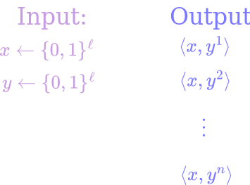
Given a truly random “seed” consisting of $x, y \in \lbrace 0,1 \rbrace^\ell$ (for $\ell$ to be specified later but spoiler that it’s gonna be $\log(n/\epsilon)$), our distribution will output $n$ bits. The $i$th bit is $\langle x, y^i \rangle$ (treating $y$ as an element of $\mathbb{F}_{2^\ell}$ for the purposes of exponentiation). That’s it, that’s the construction.

To see that this works, fix any non-empty subset $S \subseteq [n]$. By linearity, $\sum_{i \in S} \langle x, y^i\rangle = \langle x, \sum_{i \in S} y^i\rangle$. So, we want to show that
\[1/2 - \epsilon \leq \Pr_{x, y} \Big[\langle x, \sum_{i \in S} y^i\rangle \equiv 1 \text{ mod 2}\Big] \leq 1/2 + \epsilon .\]Imagine first choosing $y$. If $\sum_{i \in S} y^i \neq 0$, then the sum in question will be odd with probability exactly $1/2$ (to see this, choose an index where $y$ is nonzero, and then condition on the value of $x$ on every other index – now the overall parity is entirely determined by that one remaining bit of $x$). So, it suffices to show that
\[\Pr_y\Big[ \sum_{i \in S} y^i = 0\Big] \leq \epsilon.\]Well, $\sum_{i \in S} y^i$ is a non-zero polynomial of degree at most $n$, so it has at most $n$ roots. So, as long as we choose $\ell$ such that $n / 2^\ell \leq \epsilon$, this will be satisfied. We can choose $\ell = \log(n/\epsilon)$ as promised.
Fooling Width-2 Branching Programs
Ok, that was super neat! But it’s maybe not clear what this has to do with “tricking algorithms with only 1 bit of memory”. Let me try to convince you we can also do that.
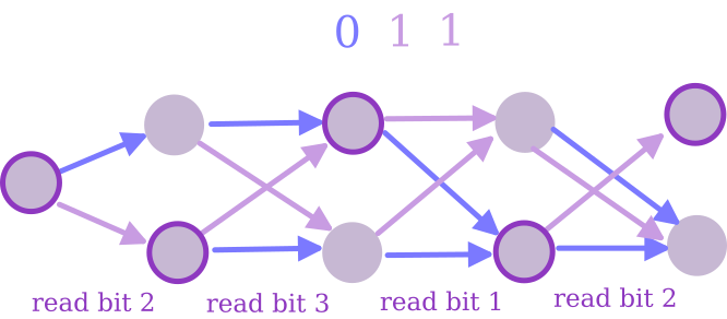
The model we want to trick consists of width-2 Branching Programs. Each of these guys has a list of $n$ indices, and two memory states. When he wakes up on the $i$th day, he finds the $i$th index in his list, looks at that index of your string, and then comes up with a new memory state based on his old memory state and that bit.

Note that this is maybe a little stronger than “algorithm with 1 bit of memory” sounds, since he’s allowed to know what day it is, and have different rules for how to update memory depending on the day1. By “tricking” these guys, I mean that I want a distribution $\mathcal{X}$ with the property that, for any width-2 branching program, the probability that he finally ends up in the first state when given an output of $\mathcal{X}$ is within $\epsilon$ of the probability when given a truly random $n$-bit string.
It turns out that small-bias sources do the job. An argument is given in this paper, which I’ll explain below. It’s easiest to talk about in Fourier basis (which means that it’s also easier to think of bits as being $\lbrace -1, 1\rbrace$ instead of $\lbrace 0, 1\rbrace$ – will do this from now on). Recall that we can express any function $\lbrace -1,1 \rbrace^n \to \lbrace -1, 1 \rbrace$ as $\sum_{S \subseteq [n]} a_S \prod_{i \in S} x_i$, where we call the values of $a_S$ the “Fourier coefficients”.
Lemma: Let $f: \lbrace -1, 1\rbrace^n \to \lbrace -1, 1 \rbrace$ be computed by a width-$2$, length-$t$ branching program. That is, $f(x) = -1$ if the program ends up in the first state after reading $x$, and $1$ if it ends up in the other state. Then, $f$’s Fourier coefficients have $L_1$ norm at most $t$ – that is, $\sum_{S \subseteq [n]} \vert a_S\vert \leq t$.
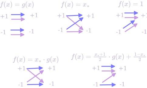
Proof: By induction, the state after $(t - 1)$ steps is described by a function $g$ whose Fourier transform has $L_1$ norm at most $(t-1)$. Now, there’s 16 different possibilities for what the last step of the branching program could look like; we just need to show that none of them increase the $L_1$ norm by more than 1. Let $x_*$ be the bit that gets read on the $t$th day; here’s a runthrough of 5 of the cases (the rest are symmetric – you can check if you really want):

Except for the last one, none of these can increase the $L_1$ norm of the Fourier transform. In the last one, there are 2 terms of norm $\vert \vert g(x)\vert \vert /2$, and 2 terms of norm $1/2$, so their sum has norm at most $\vert \vert g(x)\vert \vert + 1 \leq t$. $\hspace{20 px}\square$
Lemma: For any $f$ with $\sum_{S \subseteq [n]} \vert a_S\vert \leq t$, and any $\epsilon$-biased distribution $\mathcal{X}$, $\Big\lvert \Pr\Big[f(\mathcal{X}) = 1\Big] - \Pr\Big[f(\mathcal{U_n}) = 1\Big]\Big\rvert \leq t \epsilon$. That is, the behaviour of $f$ on $\mathcal{X}$ is at most $t\epsilon$ different from its behaviour on true randomness.
Proof: The expected value of $f$ on uniform random input is given by $a_{\emptyset}$, so it suffices to show that $\Big\lvert \mathbb{E}\sb{x\gets\mathcal{X}}\Big[\sum_{S \subseteq [n], S \neq \emptyset} a\sb{S} \prod\sb{i \in S} x^i\Big] \Big\rvert \leq t\epsilon$. By linearity of expectation, we can write
\[\mathbb{E}\sb{x\gets\mathcal{X}}\Big[\sum\sb{S \subseteq [n], S \neq \emptyset} a\sb{S} \prod\sb{i \in S} x^i\Big] = \sum\sb{S \subseteq [n], S \neq \emptyset} a\sb{S} \Big(\mathbb{E}\sb{x\gets\mathcal{X}}\Big[\prod\sb{i \in S} x^i \Big]\Big).\]Since $\mathcal{X}$ is $\epsilon$-biased, each of these expectations will be at most $\epsilon$ in magnitude. So, we have
\[\Big\lvert \sum\sb{S \subseteq [n], S \neq \emptyset} a\sb{S} \Big(\mathbb{E}\sb{x\gets\mathcal{X}}\Big[\prod\sb{i \in S} x^i \Big]\Big)\Big\rvert \leq \epsilon \cdot \sum\sb{S \subseteq [n], S \neq \emptyset} \vert a\sb{S}\vert \leq t \epsilon. \hspace{20 px}\square\]So, if $t$ is polynomial in $n$, using our small-bias distribution above we can choose $\leq 1/(1000t)$ to trick the program very well with seed length only $\ell = \log(n/\epsilon) = \mathcal{O}(\log n)$. Good for us! Unfortunately, it turns out that figuring out how to do this kind of thing for width 3 branching programs is much much trickier – and for width 4 branching programs we really just don’t know. Tune in next time!
-
Also note that we’re talking about general branching programs here. In the future, we’ll really care mostly about read-once branching programs – i.e. branching programs that never revisit the same index of your string twice (and in fact we’ll often just assume the program reads the bits of the string in order). But these arguments work either way, so figured might as well state in generality. ↩