Lost in Space II
Alright, last time was a good derandomization warm-up. We saw that, for the purposes of tricking width-2 ROBPs (a kind of “non-uniform” version of algorithms with only 1 bit of memory), we could make $\mathcal{O}(\log n)$ bits of true randomness look like $n$ bits. But, if our real goal is to understand to what extent we can simulate random algorithms deterministically, this is pretty disappointing – most of the algorithms I care about definitely use more than $1$ bit of memory. So let’s go beyond 1 bit, and ask “if a problem can be solved by a randomized algorithm with $s$ bits of space, how many bits of space do we need to solve the same problem deterministically?”1.
Savich’s Theorem
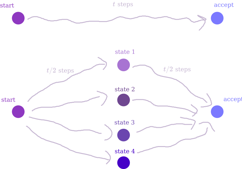
It turns out that $\mathsf{BPSPACE}(s) \subseteq \mathsf{SPACE}(s^2)$. The idea is pretty simple and also shows that $\mathsf{NSPACE}(s) \subseteq \mathsf{SPACE}(s^2)$ – if you’re in my target audience, you’ve maybe seen this before. The first thing to note is that, when limited to $s$ space, the algorithm can only run for at most $\mathcal{O}(2^s)$ steps2. So, if for every $t$ I could answer the question “what’s the probability that the algorithm goes from some memory configuration $C$ to a different configuration $C’$ after $t$ steps”, I would be cooking – set $t = 1000 \cdot 2^s$, $C$ to be the initial configuration, and enumerate over all accepting configurations $C’$ to calculate the overall acceptance probability.
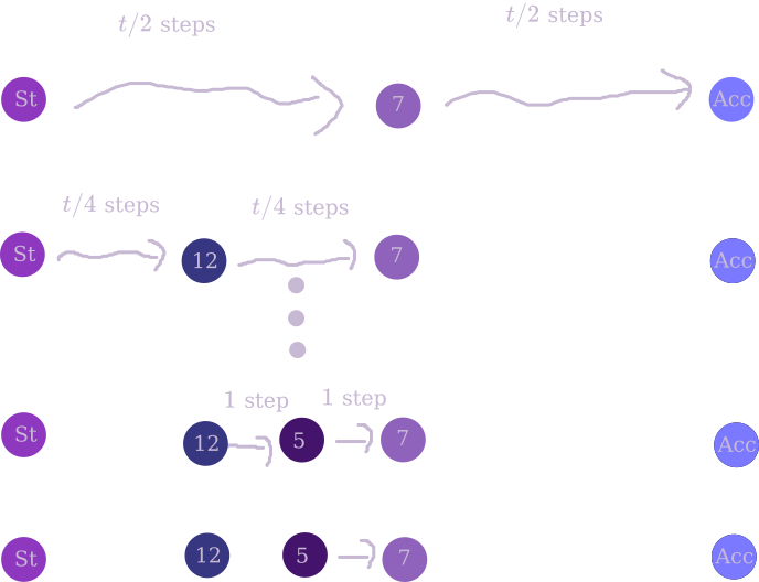
Answering this question for $t = 1$ is pretty easy – just look at the transition probabilities for one step of the algorithm. Now, suppose I have a good algorithm to solve it for $t/2$ steps, and wanna figure out $t$. Well, we can enumerate over all possibilities for a memory configuration $C_{mid}$, and for each one multiply the probabilities of going from $C \to C_{mid}$ in $t/2$ steps and going from $C_{mid} \to C’$ in $t/2$ steps – summing over all $C_{mid}$ gives the probability of going $C \to C’$ in $t$ steps.

In addition to the space required to run the $t/2$ version of the algorithm, we only need $s$ bits to remember $C_{mid}$. So, by induction, we can solve the whole problem in $\log(2^s) \cdot s = s^2$ space3.

There’s another way of thinking about this algorithm in terms of matrix exponentiation. Thinking of your algorithm as a $2^s$-state finite automaton, you can imagine writing down a $2^s \times 2^s$ matrix $M$ representing its transition probabilities in a single step. Now, if you could compute any desired entry of $M^t$, you could find the probability that the automaton is in an accepting state after $t$ steps.
- You can find any entry of the original matrix $M$ with like no space overhead, just by looking at the algorithm.
- If you can compute any entry of $M^{k}$, you can compute any entry of $M^{2k}$ with only $\mathcal{O}(s)$ more bits of overhead – in addition to the space required to compute an entry of $M^{k}$, you’ll need enough space to store the values of two entries and their product, a counter for what index in the matrix row you’re looking at, and a total. Or something like that.
- So, you can compute any entry of $M^{2^s}$ with only $\mathcal{O}(s\log(2^s)) = \mathcal{O}(s^2)$ bits of memory.
Nisan’s PRG
Savich’s theorem is the reason you never hear anyone talk about “$\mathsf{BPPSPACE}$” – since a polynomial squared is a polynomial, $\mathsf{BPPSPACE} = \mathsf{PSPACE}$. However, if you’re interested in logspace, this isn’t good enough – all we’ve got is $\mathsf{BPSPACE}(\log n) \subseteq \mathsf{SPACE}(\log^2 n)$. If you’re hoping the fact that I started this section this way means I’m about to give you a better inclusion, tough luck – you’ll have to wait until the next section for that. But I will show you another proof of the same thing.
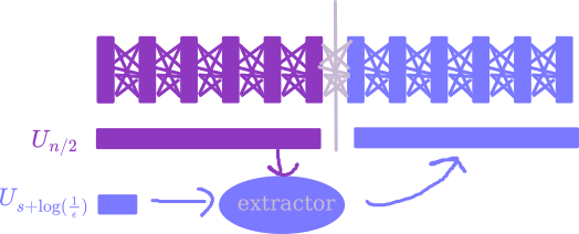
Actually that’s not really fair, because this is in many ways much stronger – a construction due to Nisan of a PRG with seed length $\mathcal{O}(s \log n)$ fooling any width-$2^s$ ROBP. The basic idea makes a lot of sense: suppose I fed you $n/2$ random bits, and then you asked me for $n/2$ more. Do I need to cook up a whole $n/2$ new bits for you? Nah, since you only remember $s$ bits about the previous stuff I gave you, as long as I mix it up a little there’s no way you’ll remember enough to know the difference when I serve it to you again.
Slightly more formally, there’s the idea of a “seeded extractor”, which I think I touched on a bit in this post. The upshot is, given a distribution with min-entropy $k$ (meaning that no specific output occurs with probability more than $2^{-k}$), as long as you also have access to a small amount of true randomness – say, $d > \log(n/\epsilon)$ bits4 – you can turn it into something $\epsilon$-close to the uniform distribution on about $k + d$ bits. Now, look at the state your branching program is in after you’ve fed it $n/2$ random bits. We can split into two cases:
- Rare states: some states might occur with probability less than $\epsilon / 2^{s}$. Since there’s only $2^s$ possible states, the chance of ending up in a rare state is at most $\epsilon$.
- Common states: suppose you end up in state $x$ after reading $n/2$ uniform random bits with probability at least $\epsilon / 2^{s}$. This means that there are at least $2^{n/2} \cdot \epsilon / 2^{s} = 2^{n/2 - s - \log(1/\epsilon)}$ different length-$n/2$ inputs leading to state $x$. So, if we take $U_{n/2}$ and condition on reaching state $x$, this distribution still has min entropy at least $n/2 - s - \log(1/\epsilon)$.
This is really nice! This means that, if you only had $n/2 + s + \log(1/\epsilon)$ bits of randomness, you could start by feeding the branching program $n/2$ bits of true uniform randomness, and then use the remaining $s + \log(1/\epsilon)$ bits as the seed of an extractor which you feed those same $n/2$ bits into again. With probability $1 - \epsilon$, you end up in a common state after the first $n/2$ bits, in which case the extractor will work and the final output distribution of the ROBP will be $\epsilon$-close to what it’s supposed to be. Overall, this means the final output distribution is $2 \epsilon$-close to what it’s supposed to be.

Nisan’s PRG comes from applying this approach recursively: in order to turn some number of random bits into twice as many pseudorandom bits, we only need to put in like $s + \log(1 / \epsilon)$ real random bits, so to generate all $n$ we should only need like $\big(s + \log(1 / \epsilon)\big) \log n$ seed bits5. This is what I promised!
If you don’t want to worry too much about extractors, you can use Nisan’s original even simpler construction: choose $x \gets U_{s}$, and then choose about $\log n$ many hash functions $h_1, \dots, h_{\log n}$ from a pairwise independent hash family $\mathcal{H}: \lbrace 0,1\rbrace^s \to \lbrace 0,1\rbrace^s$. Output $x$ with all the $2^{\log n}$ different subsets of the hash functions applied to it – i.e.
\[x, h_1(x), h_2(x), h_2(h_1(x)), h_3(x) \dots.\]In any case, we’ve got a PRG that needs seed length only $\mathcal{O}(s \log n)$. By enumerating over all possible seeds, this shows that $\mathsf{BPSPACE}(s) \subseteq \mathsf{SPACE}(s \log n)$. This is nice, but when $s = \log n$, we’re still just getting $\mathsf{BPSPACE}(\log n) \subseteq \mathsf{SPACE}(\log^2 n)$, which is no better than what Savich gave us. As we’ll see in the next section, by combining this approach with ideas from Savich’s theorem, we can get something even stronger.
Saks-Zhou
Remember how, when we talked about Savich’s Theorem, we mentioned that you can think about the problem as powering the transition matrix $M$ of a $2^s$-state DFA? Well, you might notice that we don’t actually need the exact $t$th power of the matrix – since $\mathsf{BPSPACE}$ is defined as having error probability bounded away from $1/2$, we can get away with just a pretty reasonable approximation. The key insight of Saks and Zhou was an algorithm to do this approximate powering in only $\mathcal{O}(s^{3/2})$ space, as opposed to the $\mathcal{O}(s^2)$ you’d get from repeated squaring. This shows that $\mathsf{BPSPACE}(\log n) \subseteq \mathsf{SPACE}(\log^{3/2} n)$, which is (up to a recent shaving of lower-order factors) currently the best known explicit derandomization of $\mathsf{BPL}$.
The scheme looks something like this:
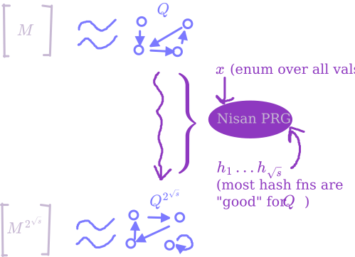
- Given a $2^s \times 2^s$ stochastic matrix $M$, we can come up with a $2^s$-state finite automaton $Q$ whose transition probabilities are a good approximation for $M$. I mean, $Q$ will read binary input, so all the entries in its transition matrix $M_Q$ are multiples of $1/2$, but given error parameter $\epsilon$ we make sure that the entries in $M_Q^{1/\epsilon}$ are very close to the entries of $M$.
- Now, note that using Nisan’s PRG with seed length $s\sqrt{s}$ will give $2^{\sqrt{s}}$ pseudorandom bits, on which $Q$ behaves approximately the same as it would on $2^{\sqrt{s}}$ real random bits. So, enumerating over all seeds to Nisan’s PRG, we can approximately compute $M^{2^{\sqrt{s}}}$.
- We really wanted $M^{2^{s}}$, so let’s take the output matrix we got from that approximate powering, and approximate power it again $\sqrt{s}$ many times to get the final output.
Alright, what did we win? For each of $\sqrt{s}$ nested calls, we had to enumerate over seeds of length $s \sqrt{s}$, bringing us to a grand total of $\sqrt{s} \cdot s \sqrt{s} = \dots s^2$? Well that’s no good.
The next observation needed (which I’m not going to explicitly prove) is that Nisan’s PRG – at least the version we talked about with pairwise independent hashes – is super friendly. Friendly in the sense that, if you fix any automaton $Q$, then for most choices of hash functions $h_1, \dots, h_{\sqrt{s}}$, you can $\epsilon$-fool $Q$ just by choosing the additional randomness of $x$. Of course, this isn’t true of all hash functions, so we can’t dispense of that randomness – but this is a nontrivial property, since you might expect the distribution only looks “spread out” appropriately when you look over all the randomness, whereas actually for most settings of almost all the randomness, it’s spread out enough just over the remaining bits.
Why is that fact useful? Well, now let’s just pick one setting of $h_1, \dots, h_{\sqrt{s}}$ and reuse it for every level of the approximate powering. We still have to do the enumeration over $x$ at each level, and of course we have to enumerate over $h_1, \dots, h_{\sqrt{s}}$ at the bottom level. But this is saving immensely on space: now, the cost is
- $\mathcal{O}(\sqrt{s} \cdot s)$ for the enumeration over $h_1, \dots, h_{\sqrt{s}}$, since each hash function takes $\mathcal{O}(s)$ bits
- $\mathcal{O}(\sqrt{s} \cdot s)$ for the enumeration over $x$ on each of $\sqrt{s}$ nested calls
so we’re feeling pretty happy! The reason this is ok is that, fixing $M$, $M^2$, $M^4$, $\dots$, the friendliness of Nisan’s PRG means that a random choice of $h_1, \dots, h_{\sqrt{s}}$ is likely to be “good” for all of them simultaneously6, by which I mean that it’ll give a good approximation when we use it to square.

That’s the post for today! Lots of cool ideas. Whenever I get around to the next chapter of this story, I’ll finally start talking about some fancy more recent stuff.
-
This post is basically just a more hand-wavey transcription of Tal’s lovely lecture notes, so you should check those out if you wanna see this in more detail. Lots of cool stuff there – will probably write at least one more post about it. tbh I don’t know that I’ve really added value to Tal’s explanation, so maybe this post isn’t achieving the goal of this blog too much – but at least writing it forced me to understand. ↩
-
Otherwise it’ll repeat a configuration, and so have the potential to loop forever. Note that while you could define $\mathsf{BPSPACE}$ so that it just has to halt eventually with probability 1, but might run forever on measure-0 events, typically you mandate that there’s no way for it to run forever. In particular, if you let have a possibility of looping forever, then it contains $\mathsf{NSPACE}$, since it can keep retrying its guesses until it gets a super unlikely coin flip sequence. But also if you’re slightly more careful with things you can analyze Savich to make it work for this definition. ↩
-
If you wanna be careful, I guess you need to think about with what precision you’re keeping track of probabilities. But you should have enough space to be pretty fine. ↩
-
I’m being imprecise with parameters here, as I am for a lot of this post. There’s lots of different interesting constructions of extractors; you can look at some of Tal’s notes linked above for a few examples. ↩
-
To make this argument precise, you need to do some kind of hybrid argument, first replacing the pseudorandom bits with actual random bits, and then applying the argument above to say you can extract to something twice as long. Also, maybe be a little careful about the $\epsilon$ there since your errors are probably adding – plugging in $\epsilon/n$ is a better idea. ↩
-
Slightly thorny issue: we’re not actually going to be calling our squaring procedure on $M^2$, we’re going to be calling it on the approximate version of $M^2$ produced by our first squaring. So, these matrices aren’t just fixed in advance things, they actually do depend to some extent on $h_1, \dots, h_{\sqrt{s}}$. To fix this issue, in the powering procedure Saks and Zhou also enumerate over all slight perturbations of matrix, which drowns out this annoying conditioning effect. ↩